Adaptive Classification and More
We use machine learning almost everywhere now, and a lot of research is focused on improving the accuracy, improving the time it takes us to train the networks, improving the complexity, etc… I would like to contribute a little to a slightly different problem: how would we improve test time figures of merit?
Suppose you are controlling a robot using a machine learning algorithm, and would like to increase its battery life. If you don’t care about the training time, but test-time accuracy is important, but not as important as your battery life – how would you go about it?
We have recently released a work on hardware of the adaptive classifiers, but I wanted to give a more “people-friendly” explanation here
You can download the iPython Notebook that I used to generate the images here.
The idea is based on selecting from multiple classifiers that differ in complexity and accuracy, such that we maximize all figures of merit at test time.
“Hardness” of a problem
Let us define “hardness” of a problem as “how easy is given problem” meaning if I have several classifiers, how complex of a classifier do I need to use to identify the label correctly.
Quick example on “Hard” problems
To visualize “hard” data points, let us look at the UCI Penbase dataset. I will use a linear classifier as a classifier for “easy” examples, because it is cheap and fast.
In the images below I show three numbers T:a/P:b/L:c. T is the true label for the image, P is the prediction of the second degree polynomial, and L is the result of a linear classifier. That means every time we see problems like these, the linear classifier will fail.
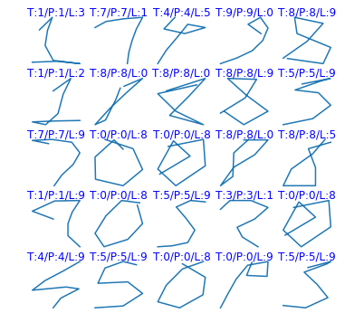
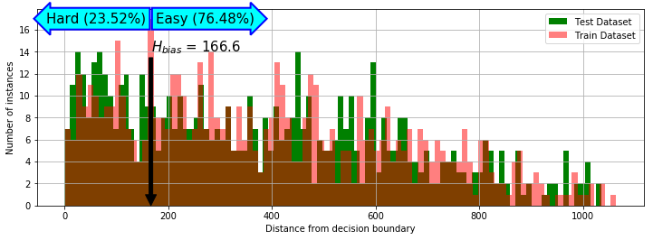
As a first order, let’s say that the “hardness” of the problem is defined as a distance from the decision boundary1. So all of the above examples would be considered “hard”.
Simple example
To visualize how the idea of “hardness” would create decision boundaries, let us consider a simpler (2D) example:
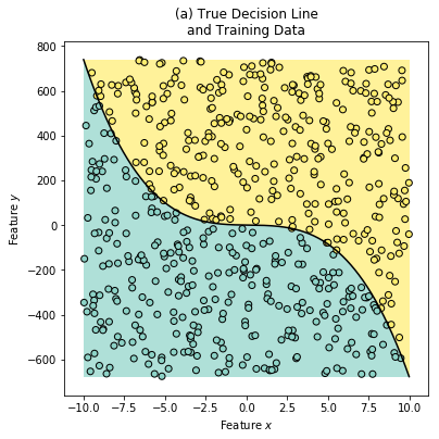
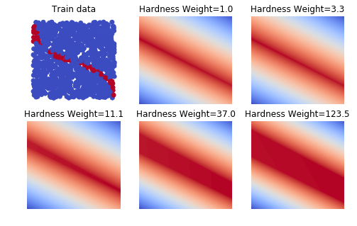
The above synthetic dataset was generated using the following True Label generator
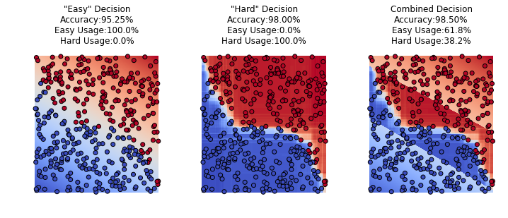
Now let’s assume that we are running on a tight energy budget, and decide to use a cheap Logistic Regression, and find out that the new equation and the plots for the Predicted Labels should be
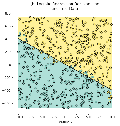
Notice that some “yellowish” labels bleed into the blue region and vice versa. The accuracy on the training data for the classifier is 94%.
To separate the hard data points from the easy ones, we will compute the hard_bias as follows2:
where is an indicator function. Now we can specify the boundaries for the Hardness Pseudo-Labels:
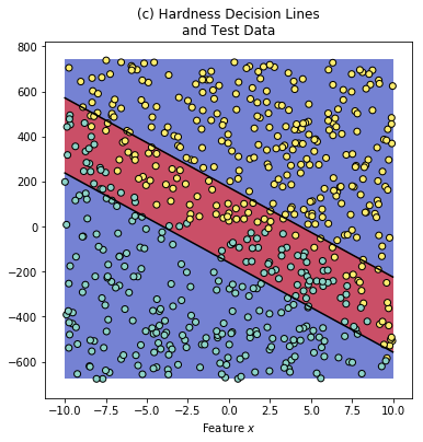
If we analyze the test and train synthetic data, we find out that only a fraction of all the data points require complex classification.
Chooser Function
in order to choose if we want to use a more expensive classifier or not, we use a “chooser” function – another logistic regression function which would predict the “hardness” of the problem. As a first order approximation we will define the chooser as follows:
Step 1. Create hardness pseudo-labels
1
2
3
4
5
6
7
8
9
10
11
12
13
14
15
16
17
18
19
20
21
22
23
24
25
## Preprocessing stage

# Predict the easy $$y'$$ and find out which ones of them are wrong
y_prime_easy = easy.predict(X_train)
wrong = y_prime_easy != y_train

# Compute the regression lines
a = -easy.coef_[0][0] / easy.coef_[0][1]
b = -easy.intercept_[0] / easy.coef_[0][1]
y_prime_easy_regr = X_train[:, 0]*a + b

# Get the bias and compute the pseudo labels
y_decision_hard_up = y_prime_easy_regr + H_bias
y_decision_hard_down = y_prime_easy_regr - H_bias

hard = np.logical_and(X_train[:,1] < y_decision_hard_up, X_train[:,1]  > y_decision_hard_down)

# Create a "hardness" envelope
y_pseudo_1 = -np.ones(y_train.shape)
y_pseudo_1[X_train[:,1] < y_decision_hard_up] = 1
y_pseudo_2 = -np.ones(y_train.shape)
y_pseudo_2[X_train[:,1] > y_decision_hard_down] = 1

y_pseudo = -np.ones(y_train.shape)
y_pseudo[hard] = 1
Step 2. Train the “chooser”
1
2
3
4
5
6
7
8
9
10
chooser = [LinearSVC(), LinearSVC()]
chooser[0].fit(X_train, y_pseudo_1)
chooser[1].fit(X_train, y_pseudo_2)

def chooser_predict(X):
  hardness = chooser[0].predict(X)*chooser[1].predict(X) # Has to be -1/+1
  combine = np.zeros(hardness.shape)
  combine[hardness == -1] = easy.predict(X[hardness == -1])
  combine[hardness == 1] = hard.predict(X[hardness == 1])
  return combine
Improvement on decision boundaries
We have described above that we create a linear “bias” to separate the hardness, but in reality we can just use incorrectly classified samples as a class, and train the classifier and let it create the boundaries automatically.
Theory
| Given | Description |
|---|---|
| Input data / labels | |
| Collection of classifiers | |
| Cost associated with classifiers | |
| “Chooser” function |
| Where | Description |
|---|---|
| Input space | |
| Collection of output Labels | |
| Upper bound on the budget |
Need to train the “chooser” such that
The equation basically says
Find a setting for a “chooser” function such that from all given (pre-trained) classifiers chooses the one that correctly classifies the current input, while maintaining the budget
In the code we will not take the budget into account, and will control it only by the class weight as shown below. This is done for simplicity, and because we don’t have actual numbers on how much more complex the “hard” classifier is.
Step 1. Train the easy and a hard classifier
1
2
3
4
5
# X_train, y_train are the training samples
easy_train = easy.predict(X_train)
hard_train = hard.predict(X_train)
y_pseudo_auto = np.zeros(y_train.shape)
y_pseudo_auto[easy_train == y_train] = easy_train[easy_train == y_train]
Step 2. Choose the proper Hyperparameters and run the tests
Decide on the “Weight” of the Hard classes. This is the same as the class weights in the SVMs. This is important because the “hardness” of the classes is a highly skewed classification.
For example, the plots below show how the decision on hardness change with different weight on the “hard” class.
We can also see the utilization at every different setting for the hardness weight hyperparameter:
1
2
3
4
5
6
7
8
9
10
11
12
13
14
15
16
17
18
19
class_weights = {-1: 1., +1: 1, 0: 1}

for _ in xrange(10):
  chooser_auto = LinearSVC(class_weight = class_weights)
  chooser_auto.fit(X_train, y_pseudo_auto)

  cls_to_use = chooser_auto.predict(X_test)
  # cls_to_use = 2*np.abs(cls_to_use) - 1

  y_adaptive = np.zeros(cls_to_use.shape)
  y_adaptive[cls_to_use == 1] = easy.predict(X_test[cls_to_use == 1])
  y_adaptive[cls_to_use == -1] = easy.predict(X_test[cls_to_use == -1])
  if np.sum(cls_to_use == 0) > 0:
    # print "Found zeros"
    y_adaptive[cls_to_use == 0] = hard.predict(X_test[cls_to_use == 0])

  print "Test Accuracy @ hard weight = {:.1f} : {:.2%}".format(class_weights[0], np.mean(y_adaptive == y_test))
  print "\tHard Utilization: {:.2%}".format(np.mean(cls_to_use == 0))
  class_weights[0] *= 3.
1
2
3
4
5
6
7
8
9
10
11
12
13
14
15
16
17
18
19
20
Test Accuracy @ hard weight = 1.0 : 95.25%
  Hard Utilization: 0.00%
Test Accuracy @ hard weight = 3.0 : 95.25%
  Hard Utilization: 0.00%
Test Accuracy @ hard weight = 9.0 : 96.00%
  Hard Utilization: 1.00%
Test Accuracy @ hard weight = 27.0 : 98.00%
  Hard Utilization: 14.25%
Test Accuracy @ hard weight = 81.0 : 97.75%
  Hard Utilization: 23.25%
Test Accuracy @ hard weight = 243.0 : 98.25%
  Hard Utilization: 28.50%
Test Accuracy @ hard weight = 729.0 : 98.25%
  Hard Utilization: 31.25%
Test Accuracy @ hard weight = 2187.0 : 98.25%
  Hard Utilization: 31.75%
Test Accuracy @ hard weight = 6561.0 : 98.50%
  Hard Utilization: 32.75%
Test Accuracy @ hard weight = 19683.0 : 98.50%
  Hard Utilization: 33.00%
-
Note that this is not really true. There are cases where the problem is very far from decision boundary, but is still misclassified, and vice-versa ↩
-
This
biasis only for illustration purposes, in reality the “hardness” is subject to a little more complex decision making process. In particular is an appropriate function to train a “chooser” function with respect to loss ↩